Paolo Pinto
Aeronautical
Engineer and Computer Programmer
The Pacejka Equation
Since
the ‘70s Dr. Pacejka has been developing several tyre behaviour models which
led to the “Magic Formula” : a function simulating with relative simplicity and
good approximation the main tyre characteristics.
The
Magic Formula is a transcendent function :
Y(x) = D sen(C arctan(Bx – E [ Bx – arctan(Bx) ] )
where B,C,D,E are coefficients. relevan
The
x, y variables can be associated from time to time to different parameters ;
for example :
x =
slip angle , y = Fy if studying the tyre’s ability to provide centripetal
force
x =
slip ratio , y = Fx for the tractive force
It
is also possibile to take into account
camber, ply steer and conicity, with slight modifications..
The
function actually has the near-magic property of being useful for simulating
many different tyre phenomena just by changing the coefficient and the meanings
of x, y.
Function
study
The
Y(x) function is anti-symmetric ; it always goes through the axis’ origin and
it always has there a null second derivative.
In
tyre models y’(0) >0 is always
desiderable ; it is possibile to demonstrate that this implies B,C being of the
same sign.
For
the same reason it must always be y’’’(0) < 0 ; this implies
E > -(1 + C2/2)
The
curve always shows an horizontal asymptote for x tending to infinity.
The
asymptote’s value is :
D
sen(Cp/2) if E <1
D
sen (C arctan (p/2)) if E =1
-D
sen (Cp/2) if E >1
As a
consequence, the need to have y(x)>0 for x tending to infinity leads to
coefficients :
E<1 ; 0 <C <2
It
must be said that several other different couples of values for E, C could suit this need.
The B parameter
B is
called Stiffness Factor
It
controls the slope of the curve at the origin ; in practical models it must
always be B>0
It
must be pointed out that B also exerts a strong influence on the relative
minimum and maximum position
The C parameter
C is
called Shape Factor
The
possible presence of a relative maximum (a “peak” in NON mathematically correct
terms) on the right of the zero depends on C being >1 (provided the
previously stated conditions are met) .
This
maximum happens at am ; a position which may be obtained from :
B(1-E) am + E arctan(Bam) = tan (p/(2C)) (*)
The
bigger the value of C, the more pronounced the maximum.
Typical
values for C are 1.3 for the centripetal force simulation and 1.6 for the
tractive force simulation
The D parameter
D is
also called Peak Value
It
constitutes a superior limit to the function’s values, since the factor : .
sen(C
arctan(Bx – E [ Bx – arctan(Bx) ] )
cannot
obviously exceed 1 .
The E parameter
E is
also called Curvature Factor; it is usually set at a value less than zero. As
the absolute value of E goes down the
curve assumes a flatter shape
PHISICAL
APPLICATION
Not
many data are available in technical literature about the real tyres’
characteristics, expecially about race tyres.
Although
this is understandable for the latest developements, this desolating scarcity
is the same even for 20 years old designs.
When
data are available they are often only partial : for example in [2] the Lateral
Force vs Slip Angle plots stop at a =
6°, and only 4 different values of
vertical load are considered.
This
makes the Magic formula useful to those wanting to create a race vehicle
simulation., since it allows to extend the tyre behaviour to the whole range of
slip angles and vertical loads, once that the parameters are set to match a
limited quantity of experimental data.
Obviously it will be impossible to have a
perfect match ; one must also consider that all of the analytical formulas (and
many numeric solutions too) used in Engineering are useful only to give a first
approximation, to the Experimental Engineers delight.
Another application of the curves is the
simulation of tyre for which no data is available at all, by making use of the
ones of similar tyres.
For
example, if wanting to simulate a tyre similar to a given one, but a softer compound, it will often be enough
to raise the value of D.
This because (AS A RULE OF THUMB…) , B,C,E
depend on the carcass’ construction, while D depends on the compound.
If it
is desired a tyre able to give the pilot a very clear warning of the limit’s
approaching (as in videgames, where a lack of the acceleration input ought to
be compensated by an enhanced visual input), the parameters of choice are C and
E, since they rule on the adherence’s fall after the maximum.
A wider (and hence stiffer) tyre can be
simulated by an increase of B, which
will increase the initial slope. In this case it will also be useful a decrease
in C, to diminish the BCD parameter on which the peak adherence slip angle
depends.
The
Pacejka curves are here used to plot the various a,m diagrams , i.e. slip angle a versus adherence
coefficient m, at varying vertical loads FZ
It must be said that this kind of approach is
not very common in literature, since usually the centripetal force is plotted,
instead of the adherence coefficient.
The two values are anyway linked by a
proportionality factor, thereby legitimating this change.
It won’t be unuseful to remember that
“adherence factor” is not an exceedingly formally correct term , since it would
be more orthodox to refer to a “normalized force” Fy/Fz
The
easy understanding of m will anyway led to its use in these pages.
D coefficient variability under vertical load
In
starting the calculations for a complete tyre, the first value to be fixed
should be D, wich takes into account
the adherence factor.
For a Formula One tyre, a value of 1.8 under a vertical load of 600 kg will be in the
ballpark
It is very important to make D dependent on
the vertical load Fz , since the maximum adherence value depends on
it.
A good formula, presented (in different
ways) in [2] and [3] , will be
:
m = a1 Fz + a2 (**)
where
a1<0 ; a2>0
It ought to be pointed out that the nonetheless
interesting paper [3] suggests (Chapter
24) positive values for both these coefficients, a statement not congruent with
experimental data.
As an alternative it can be used the formula
shown in [4] :
m = m0 / (1+mtFz) (***)
Of
course the right coefficient must be found; referring to the experimental
values given (in a different form) for a Goodyear front F1 tyre in [2], after a
brief comparative analysis it is
observed that (**) provides a better match, at least for this kind of tyre.
Plausibile values for the coefficients are :
a1 = -00138
a2 = 1.988
where FZ is measured in Kg
To all practical effects D is the adherence
factor under a zero vertical load; the ample variability of D under load (it
can easily vary between 1.8 and 1.2) helps understanding how far are the tyre’s
adherence mechanics from the simple Couloumbian model
Cornering stiffness variability under load
Cornering stiffness is normally meant as dFy/da ; in this paper it will be meant as dm/da .
The value dFy/da increases with the vertical
load; yet dm/da decreases with Fz.
Slip angle stiffness depends on thje
vertical load by the formula :
BCD
= a3 sen (2 arctan(FZ/a4))
By
all practical means this leads to intervene on
B and C , since D is chosen on
different grounds.
Yet
it is important that the value of D be the one appropriate for the given load .
Unfortunately,
it is not possible to use equation (*) to close the algebraic system, since
this would introduce the new variable E.
The
best approach would of course be a numerical one, which finds the best B,C,E
triplet ; yet many numerical solution benefit from reasonably accurate starting
values.
Now,
some hints are given for C, at least : as previously stated its value ought to
be comprised beetween 0 and 2 ; Ref. [1] quotes 1.3 as a good value
(although it is not stated which kind of tyre was examined to determine this)
So
it will be, at least for a first evaluation
C =
1.3
The
previous formula can therefore be rewritten as :
B =
(a3 sen (2 arctan(FZ/a4))) / (C (a1 Fz + a2))
The values to research are a3 and a4 , since all
other parameters are set.
Once
again it is possible to refer to the experimental values
The a4 parameter controls the
diagram bending , while a3
is an intensity term.
Reasonable starting values can be :
a3 = 1.37
a4 = 120
where vertical load is expressed in Kg.
The
maximum’s position
As a check it is possibile to observe what
happens to am when the load increases ; it should increase too.
Let’s remember its value is given by :
B(1-E) am + E arctan(Bam) = tan (p/(2C)) (*)
A
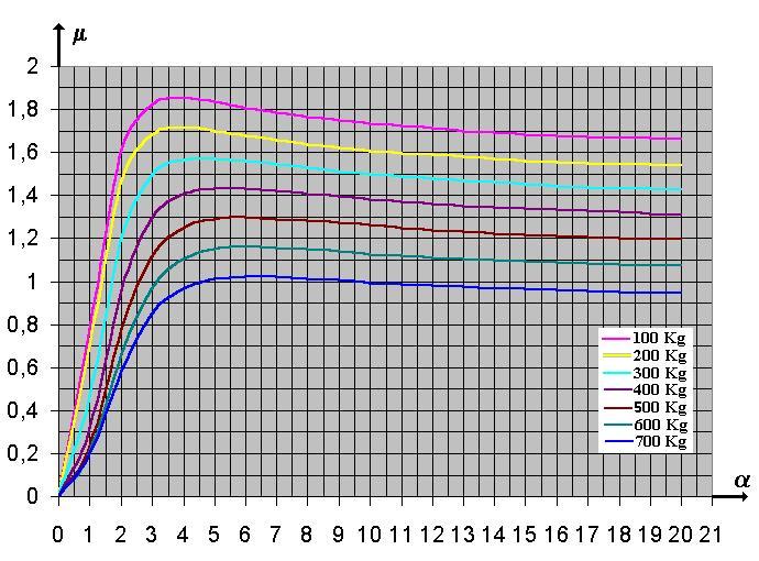
PRACTICAL EXAMPLE
Here
is a plot of Pacejka’s curves for a tyre of the following characteristics ,
under different vertical loads:
|
C |
1,35 |
|
E |
-0,4 |
|
a1 |
-0,00138 |
|
a2 |
1,988 |
|
a3 |
1,37 |
|
a4 |
120 |
Adherence coefficient
vs Slip Angle for a front F1 tyre
Glossary
Fx
: force acting along the road in a direction orthogonal to the wheel axis
Fy :
force acting along the road in the
wheel’s axis’ direction
FZ :
Vertical load on the tyre
am = slip angle of maximum adherence
a =
slip angle
m =
adherence factor
Bibliografia :
[1] M. Guiggiani : Dinamica del veicolo ; Città
Studi Edizioni
[2]
M. Milliken, D.Milliken : Race Car Dynamics ; SAE
[3]
Brian Beckman ; The Phisics of Racing ; Online Document
[4]
G.Rimondi, P.Gavardi ; A new
interpolative model of the mechanical characteristics of the tyre as an input
to handling models ; Rivista ATA 6/7/1991